Varying Model Components in ModelChain

This example demonstrates how changing modeling components within pvlib.modelchain.ModelChain affects simulation results.

Using the same PV system and weather data, we create two ModelChain instances that differ only in their temperature model. By comparing the resulting cell temperature and AC power output, we can see how changing a single modeling component affects overall system behavior.

Varying ModelChain components

Below, we create two ModelChain objects with identical system definitions and weather inputs. The only difference between them is the selected temperature model. This highlights how individual modeling components in ModelChain can be swapped while keeping the overall workflow unchanged.

import pvlib
import pandas as pd
import numpy as np
import matplotlib.pyplot as plt

Define location

We select Tucson, Arizona, a location frequently used in pvlib examples due to its strong solar resource and available TMY data.

latitude = 32.2
longitude = -110.9
location = pvlib.location.Location(latitude, longitude)

Generate clear-sky weather data

We generate clear-sky irradiance using pvlib and create a varying air temperature profile instead of using constant values.

times = pd.date_range(
    "2019-06-01 00:00",
    "2019-06-07 23:00",
    freq="1h",
    tz="Etc/GMT+7",
)

# Clear-sky irradiance
clearsky = location.get_clearsky(times)

# Create a simple daily temperature cycle
temp_air = 20 + 10 * np.sin(2 * np.pi * (times.hour - 6) / 24)

weather_subset = clearsky.copy()
weather_subset["temp_air"] = temp_air
weather_subset["wind_speed"] = 1

Define a simple PV system

To keep the focus on the temperature model comparison, we define a minimal PV system using the PVWatts DC and AC models. These models require only a few high-level parameters.

The module DC rating (pdc0) represents the array capacity at reference conditions, and gamma_pdc describes the power temperature coefficient.

For the temperature model parameters, we use the sapm values for an open-rack, glass-glass module configuration. These parameters describe how heat is transferred from the module to the surrounding environment.

module_parameters = dict(pdc0=5000, gamma_pdc=-0.003)
inverter_parameters = dict(pdc0=4000)

temperature_model_parameters = (
    pvlib.temperature.TEMPERATURE_MODEL_PARAMETERS["sapm"]
    ["open_rack_glass_glass"]
)

system = pvlib.pvsystem.PVSystem(
    surface_tilt=30,
    surface_azimuth=180,
    module_parameters=module_parameters,
    inverter_parameters=inverter_parameters,
    temperature_model_parameters=temperature_model_parameters,
)

ModelChain using the sapm temperature model

First, we construct a ModelChain that uses the sapm temperature model. All other modeling components remain identical between simulations.

This ensures that any differences in the results arise solely from the temperature model choice.

temperature_model_parameters_sapm = (
    pvlib.temperature.TEMPERATURE_MODEL_PARAMETERS["sapm"]
    ["open_rack_glass_glass"]
)

system_sapm = pvlib.pvsystem.PVSystem(
    surface_tilt=30,
    surface_azimuth=180,
    module_parameters=module_parameters,
    inverter_parameters=inverter_parameters,
    temperature_model_parameters=temperature_model_parameters_sapm,
)

mc_sapm = pvlib.modelchain.ModelChain(
    system_sapm,
    location,
    dc_model="pvwatts",
    ac_model="pvwatts",
    temperature_model="sapm",
    aoi_model="no_loss",
)

mc_sapm.run_model(weather_subset)

ModelChain:
  name: None
  clearsky_model: ineichen
  transposition_model: haydavies
  solar_position_method: nrel_numpy
  airmass_model: kastenyoung1989
  dc_model: pvwatts_dc
  ac_model: pvwatts_inverter
  aoi_model: no_aoi_loss
  spectral_model: no_spectral_loss
  temperature_model: sapm_temp
  losses_model: no_extra_losses

ModelChain using the Faiman temperature model

Next, we repeat the same simulation but replace the temperature model with the Faiman model.

No other system or weather parameters are changed. This illustrates how individual components within ModelChain can be varied independently.

temperature_model_parameters_faiman = dict(u0=25, u1=6.84)

system_faiman = pvlib.pvsystem.PVSystem(
    surface_tilt=30,
    surface_azimuth=180,
    module_parameters=module_parameters,
    inverter_parameters=inverter_parameters,
    temperature_model_parameters=temperature_model_parameters_faiman,
)

mc_faiman = pvlib.modelchain.ModelChain(
    system_faiman,
    location,
    dc_model="pvwatts",
    ac_model="pvwatts",
    temperature_model="faiman",
    aoi_model="no_loss",
)

mc_faiman.run_model(weather_subset)

ModelChain:
  name: None
  clearsky_model: ineichen
  transposition_model: haydavies
  solar_position_method: nrel_numpy
  airmass_model: kastenyoung1989
  dc_model: pvwatts_dc
  ac_model: pvwatts_inverter
  aoi_model: no_aoi_loss
  spectral_model: no_spectral_loss
  temperature_model: faiman_temp
  losses_model: no_extra_losses

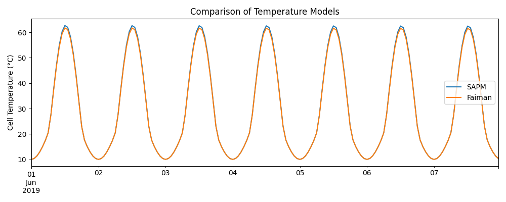
Compare modeled cell temperature

Since module temperature directly affects DC power through the temperature coefficient, differences between temperature models can propagate into performance results.

fig, ax = plt.subplots(figsize=(10, 4))
mc_sapm.results.cell_temperature.plot(ax=ax, label="SAPM")
mc_faiman.results.cell_temperature.plot(ax=ax, label="Faiman")

ax.set_ylabel("Cell Temperature (°C)")
ax.set_title("Comparison of Temperature Models")
ax.legend()
plt.tight_layout()

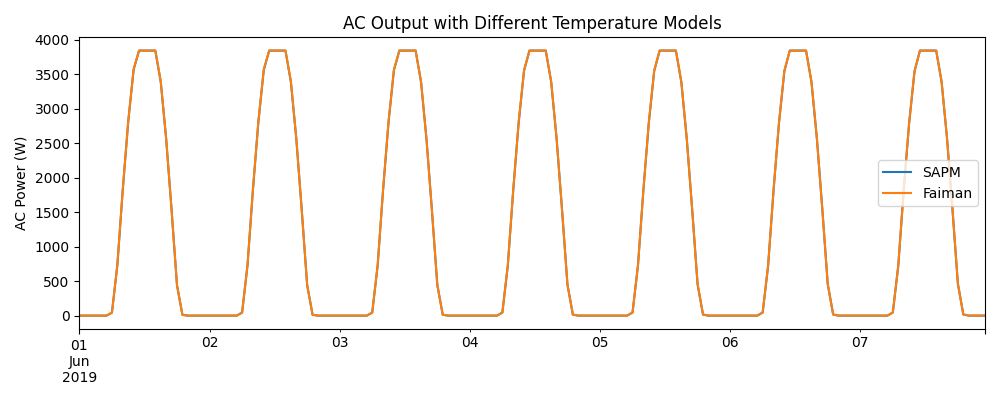
Compare AC power output

Finally, we compare the resulting AC power. Even small differences in temperature modeling can lead to noticeable differences in predicted energy production.

fig, ax = plt.subplots(figsize=(10, 4))
mc_sapm.results.ac.plot(ax=ax, label="SAPM")
mc_faiman.results.ac.plot(ax=ax, label="Faiman")

ax.set_ylabel("AC Power (W)")
ax.set_title("AC Output with Different Temperature Models")
ax.legend()
plt.tight_layout()